

SAE enrichment: which features separate two classes?
The previous two notebooks knew which concept they wanted. This one does not. Given a labeled dataset and a bank of thousands of features, which features distinguish the labels, and are they about the labels?
The answer is a warning as much as a recipe: selectivity and meaning are different properties, and the gap between them is where SAE interpretation goes wrong.
Key questions
- How do I rank thousands of features by how well they separate two classes?
- Does a feature that separates the classes necessarily encode the class concept?
- Where in a sentence does a selective feature actually fire?
Structure
- Set up
- Encode a labeled dataset
- Rank features by class selectivity
- Read what the selective features promote
- See where a feature fires
Model and data. GPT-2 small in float32 with the gpt2-small-res-jb SAE at layer 8, and 512 SST-2 sentences (stanfordnlp/sst2) labeled positive or negative.
Requirements. pip install murano-interp[sae,data,plot]
1. Set up
Section titled “1. Set up”import warnings
import plotly.io as pioimport torch
from murano import MuranoModel, Pipeline, keysfrom murano.dataset import LabeledDatasetfrom murano.plotting import ( plot_sae_feature_logit_effects, plot_sae_token_activations, save_figure,)from murano.steps import Load, SAEEncode
# The logit-effects figure carries one point per vocabulary token. Left as Plotly# JSON it makes this notebook a megabyte on disk, so render inline as a static# image; save_figure still writes the full-resolution PNG.pio.renderers.default = "png"
# sae-lens warns that this release carries loader kwargs it will not apply; the# SAE loads correctly and the warning is not actionable here.warnings.filterwarnings( "ignore", message=r"\s*This SAE has non-empty model_from_pretrained_kwargs\.", category=UserWarning,)
OUTPUT_DIR = "murano_outputs/sae_enrichment"
MODEL_ID = "openai-community/gpt2"SAE_RELEASE = "gpt2-small-res-jb"SAE_ID = "blocks.8.hook_resid_pre"N_EXAMPLES = 512
# GPT-2 is small enough that bfloat16 rounding degrades its predictions.model = MuranoModel(MODEL_ID, dtype=torch.float32)print(f"{model.model_id}: {model.n_layers} layers")openai-community/gpt2: 12 layers2. Encode a labeled dataset
Section titled “2. Encode a labeled dataset”LabeledDataset.from_hub pulls SST-2 straight off the Hub; Load and SAEEncode are the same two steps as before.
dataset = LabeledDataset.from_hub(    "stanfordnlp/sst2",    text_column="sentence",    label_column="label",    split="train",    n=N_EXAMPLES,    label_names=["negative", "positive"],)
encode = SAEEncode(model, release=SAE_RELEASE, sae_id=SAE_ID)results = Pipeline([Load(dataset), encode]).run()
record = results[keys.SAE_RECORD]labels = torch.tensor([int(label) for label in dataset.labels])print(f"{len(dataset.texts)} sentences, {int((labels == 1).sum())} positive")print(f"activations {tuple(record.activations.shape)}  [sentences, tokens, features]")
512 sentences, 266 positiveactivations (512, 53, 24576) [sentences, tokens, features]3. Rank features by class selectivity
Section titled “3. Rank features by class selectivity”Pool each feature over a sentence’s real tokens, then ask how far apart the two classes sit, in units of the feature’s own spread:
effect(f) = (mean_positive(f) - mean_negative(f)) / std(f)That is a standardized mean difference, and it is the whole ranking. Nothing here is specific to sentiment: swap the labels and the same four lines rank features for any binary split.
The BOS position is dropped. Residual-stream SAEs reliably grow a strong BOS-anchored feature which fires on every sentence, and it would otherwise dominate the pooled mean while telling us nothing about the labels.
activations = record.activations.float().cpu()tokens = record.tokens.cpu()content = record.attention_mask.bool().cpu()if model.tokenizer.bos_token_id is not None:    content = content & (tokens != model.tokenizer.bos_token_id)
per_sentence = (activations * content.unsqueeze(-1)).sum(1) / content.sum(1).clamp_min(    1).unsqueeze(-1)
positive, negative = labels == 1, labels == 0delta = per_sentence[positive].mean(0) - per_sentence[negative].mean(0)effect = delta / per_sentence.std(0).clamp_min(1e-6)
print(f"scored {effect.numel()} features")print(f"most positive-selective: #{int(effect.argmax())}  effect {effect.max():+.3f}")print(f"most negative-selective: #{int(effect.argmin())}  effect {effect.min():+.3f}")
scored 24576 featuresmost positive-selective: #16752 effect +0.375most negative-selective: #7964 effect -0.3324. Read what the selective features promote
Section titled “4. Read what the selective features promote”Ranking is cheap; interpretation is not. Project each top feature’s decoder direction
through the unembedding, exactly as sae_features.ipynb did, and read the tokens it
promotes. SAEModel.decoder hands over the whole bank at once.
decoder = encode.sae_model.decoder.float().cpu()unembedding = model.unembed_weight.detach().float().cpu()

def promoted(feature_id, k=6):    logits = decoder[feature_id] @ unembedding.T    return [model.tokenizer.decode([int(i)]).strip() for i in logits.topk(k).indices]

for name, ranked in [    ("POSITIVE-selective", effect.topk(5).indices),    ("NEGATIVE-selective", (-effect).topk(5).indices),]:    print(f"{name}:")    for feature_id in ranked.tolist():        print(            f"  #{feature_id:<6} effect {effect[feature_id]:+.3f}  {promoted(feature_id)}"        )    print()
POSITIVE-selective: #16752 effect +0.375 ['seamlessly', 'affordable', 'achievable', '2050', 'isine', '.","'] #64 effect +0.369 ['kindness', 'generosity', 'invaluable', 'gracious', 'generous', 'kindly'] #5201 effect +0.320 ['slogans', 'onyms', 'TextColor', 'Pets', 'emot', 'igraph'] #12078 effect +0.317 ['penchant', 'charisma', 'pedigree', 'temperament', 'personality', 'knack'] #6168 effect +0.281 ['ever', 'ever', 'EVER', 'anywhere', 'OPLE', 'foray']
NEGATIVE-selective: #7964 effect -0.332 ['adequately', 'timely', 'properly', 'trustworthy', 'atisf', 'responsive'] #19912 effect -0.308 ['anymore', 'nor', 'nor', 'whatsoever', 'slightest', 'anything'] #14082 effect -0.287 ['anymore', 'ever', 'ever', 'nor', 'neys', 'EVER'] #17929 effect -0.282 ['average', 'usual', 'usual', 'realizes', 'iably', 'Num'] #15591 effect -0.267 ['nothing', 'meaningless', 'nothing', 'negligible', 'insignificant', 'nowhere']Read those two lists carefully, because they are not what the ranking promised.
Some features are exactly what you would hope for: one promotes kindness, generosity, gracious; another promotes nothing, meaningless, negligible. Those are sentiment features, and the ranking found them.
But the lists also contain features that separate the classes without encoding sentiment at all:
- a negation feature (anymore, nor, whatsoever, slightest) ranks as negative-selective, because negative reviews negate more, not because negation is negative;
- a feature promoting adequately, timely, properly, trustworthy also ranks as negative-selective, since those words appear in negative reviews mainly as the thing the film failed to be;
- at least one feature promotes plain junk (TextColor, igraph), and separates the classes by accident.
Selectivity is a correlation and nothing more. A feature that separates the labels has told you it carries some signal that co-varies with them. Which signal is a separate question, and the only cheap instrument for it is the one above: look at what the feature promotes, and disbelieve the ranking when the two disagree.
5. See where a feature fires
Section titled “5. See where a feature fires”The logit lens says what a feature writes. To see what makes it read, plot its activation across the tokens of the sentences it fires on hardest.
Note which feature we plot. Not the top-ranked one, whose promoted tokens were a mixed bag, but the one two rows down whose tokens are unambiguously about sentiment. Choosing after reading, rather than trusting the rank, is the whole content of the last section; the assertion keeps that choice honest if the ranking ever shifts.
FEATURE_ID = 64
assert FEATURE_ID in effect.topk(5).indices.tolist(), (    "feature 64 fell out of the top 5; re-read the table above and pick again")
logit_fig = plot_sae_feature_logit_effects(    FEATURE_ID,    decoder=decoder,    unembedding=unembedding,    token_labels=[        model.tokenizer.decode([i]) for i in range(model.tokenizer.vocab_size)    ],    token_ids=list(range(model.tokenizer.vocab_size)),    title=f"Feature #{FEATURE_ID}: vocabulary logit effects",)save_figure(logit_fig, f"{OUTPUT_DIR}/plots/feature_logit_effects.png")logit_fig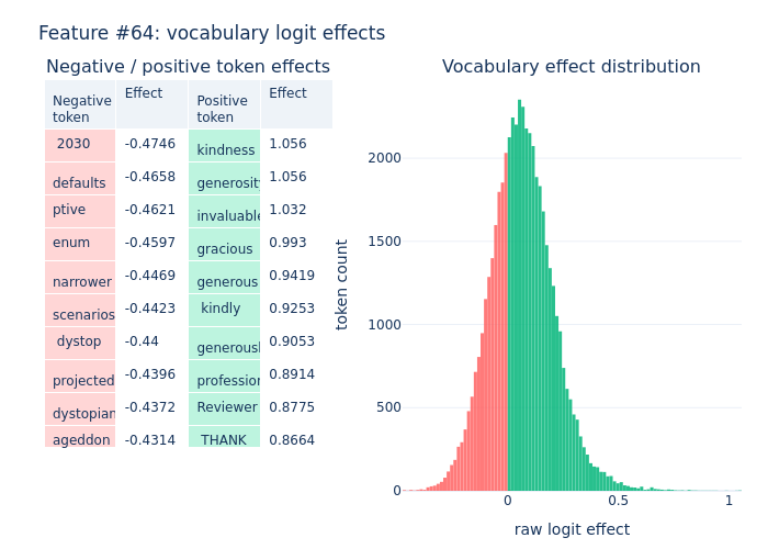
token_fig = plot_sae_token_activations( activations=activations, token_ids=tokens, attention_mask=record.attention_mask, feature_id=FEATURE_ID, decode_token=lambda token_id: model.tokenizer.decode([int(token_id)]), bos_token_id=model.tokenizer.bos_token_id, num_examples=8, title=f"Feature #{FEATURE_ID}: where it fires",)save_figure(token_fig, f"{OUTPUT_DIR}/plots/feature_token_activations.png")token_fig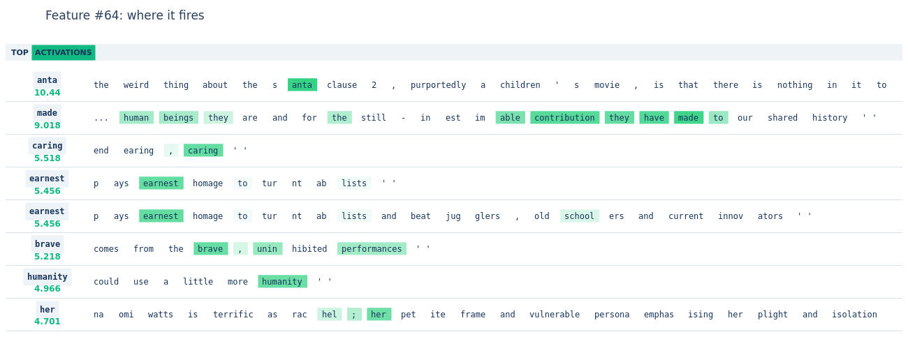
What next
Section titled “What next”sae_features.ipynbintroduces the logit lens on a decoder direction that this notebook leans on.probing.ipynbasks the same question of raw activations rather than SAE features.