Probing: where is a concept linearly readable?

A linear probe is a classifier trained on a model’s internal activations. If a simple linear model can read “positive” versus “negative” off layer 6’s residual stream, then the concept is linearly encoded there. Probe every layer and you get a map of where the information appears.

Key questions

At which layer does sentiment become linearly decodable?
Does the probe generalize, or is it memorizing?
What does the structure the probe exploits actually look like?

Structure

Set up
Train a probe per layer
Plot accuracy and the confusion matrix
Look at the structure the probe found
Did the model build the concept, or was it always there?
Save

Model and data. GPT-2 small in float32. It is small enough that bfloat16 rounding visibly degrades its predictions, so the notebooks load it explicitly in float32. 20 positive and 20 negative sentences from murano.tasks.

Requirements. pip install murano-interp[probe,plot]

1. Set up

import torch

from murano import MuranoModel, Pipeline, keys
from murano.dataset import LabeledDataset
from murano.steps import Load, Plot, Probe, Record, Save
from murano.tasks import sentiment

OUTPUT_DIR = "murano_outputs/probing"

# GPT-2 is small enough that bfloat16 rounding degrades its predictions.
model = MuranoModel("gpt2", dtype=torch.float32)
print(f"{model.model_id}: {model.n_layers} layers, {model.n_heads} heads")

gpt2: 12 layers, 12 heads

2. Train a probe per layer

Record on a LabeledDataset produces a LabeledActivationStore: activations plus the label of each example. Probe fits one classifier per layer with cv-fold cross-validation, so the reported accuracy is on held-out folds.

refit=True additionally fits a final classifier per layer on all the data and keeps it, which is what the confusion matrix below needs.

positive, negative = sentiment(n_per_class=20)
dataset = LabeledDataset.from_lists(
    texts=positive + negative,
    labels=[0] * len(positive) + [1] * len(negative),
    label_names=["positive", "negative"],
)

results = Pipeline(
    [
        Load(dataset),
        Record(model, layers="all", position="last", batch_size=8),
        Probe(cv=5, refit=True),
    ]
).run()

probe = results[keys.PROBE]
print("best layer:", probe.best_layer, "\n")
for layer, accuracy in sorted(probe.accuracy_per_layer.items()):
    spread = probe.cv_scores[layer].std()
    marker = "  <-- best" if layer == probe.best_layer else ""
    print(f"  {layer}: {accuracy:.3f} +/- {spread:.3f}{marker}")

best layer: L5.resid_post

  L0.resid_post: 0.825 +/- 0.150
  L1.resid_post: 0.850 +/- 0.146
  L2.resid_post: 0.775 +/- 0.094
  L3.resid_post: 0.850 +/- 0.122
  L4.resid_post: 0.850 +/- 0.122
  L5.resid_post: 0.925 +/- 0.061  <-- best
  L6.resid_post: 0.825 +/- 0.100
  L7.resid_post: 0.900 +/- 0.094
  L8.resid_post: 0.925 +/- 0.061
  L9.resid_post: 0.925 +/- 0.061
  L10.resid_post: 0.900 +/- 0.050
  L11.resid_post: 0.900 +/- 0.094

3. Plot accuracy and the confusion matrix

Plot draws probe accuracy per layer, with the best layer highlighted and the cross-validation spread as error bars. Because the probe kept its classifiers and the activation store is still in Results, it also draws the confusion matrix at the best layer.

Plot(output_dir=OUTPUT_DIR)(results);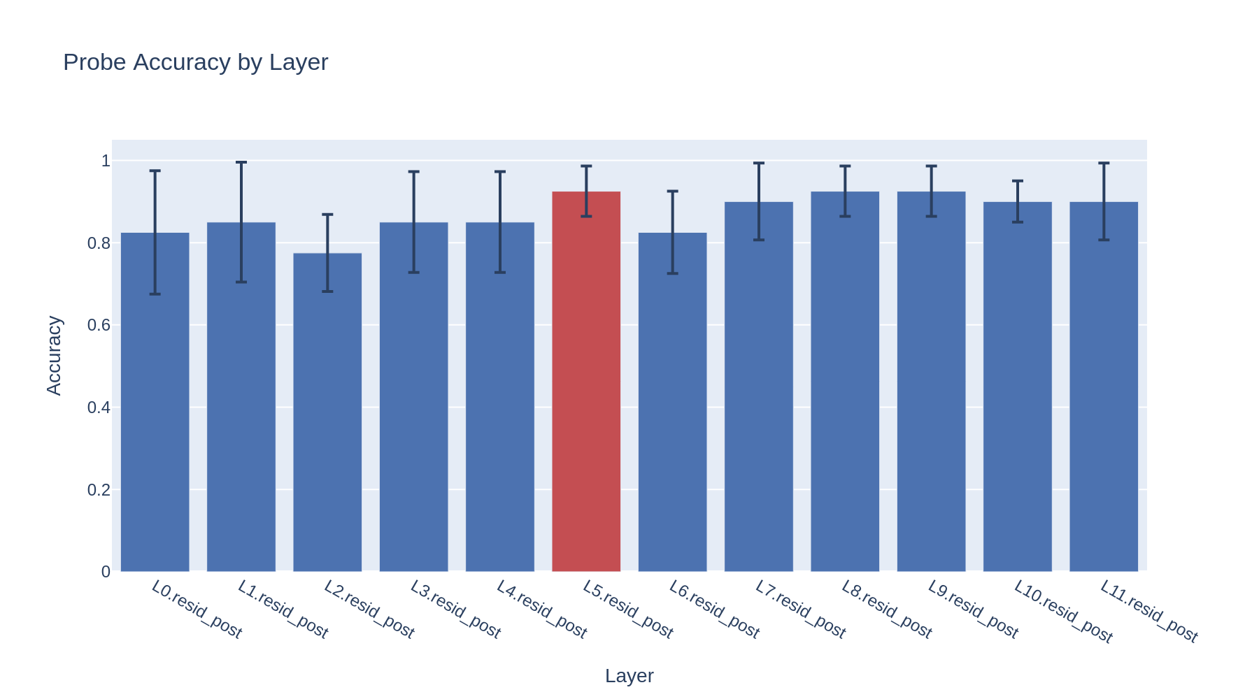

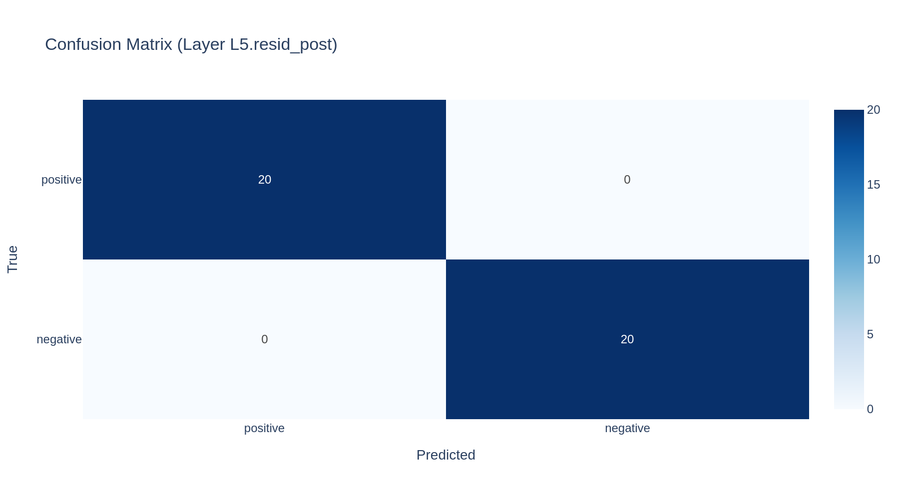
Probing: where is a concept linearly readable? figure 2

Read the confusion matrix carefully. It uses the classifier that refit=True fit on all the data, and evaluates it on that same data. It is therefore in-sample and will look flattering, often perfect. It is useful for seeing which class a probe confuses, not for estimating how well the probe generalizes.

The honest number is the cross-validated accuracy in the bar chart, where every prediction comes from a fold the classifier never saw.

4. Look at the structure the probe found

Accuracy tells you the concept is readable. It does not show you what the activations look like. plot_activation_projection reduces one layer’s activations to a couple of dimensions and scatters them by class.

It is not auto-dispatched by Plot, because it needs you to choose a layer and a reducer. You supply any scikit-learn-style reducer, so the choice of method stays yours.

LDA is supervised: it finds the axis that best separates the labels. One component is enough, so the classes are fanned out vertically only to keep the points from overlapping.

from sklearn.discriminant_analysis import LinearDiscriminantAnalysis

from murano.plotting import plot_activation_projection, save_figure

store = results[keys.RECORD]

fig = plot_activation_projection(
    store,
    probe.best_layer,
    LinearDiscriminantAnalysis(n_components=1),
    label_names=dataset.label_names,
    title="LDA (supervised)",
)
save_figure(fig, f"{OUTPUT_DIR}/plots/projection_lda.png")
fig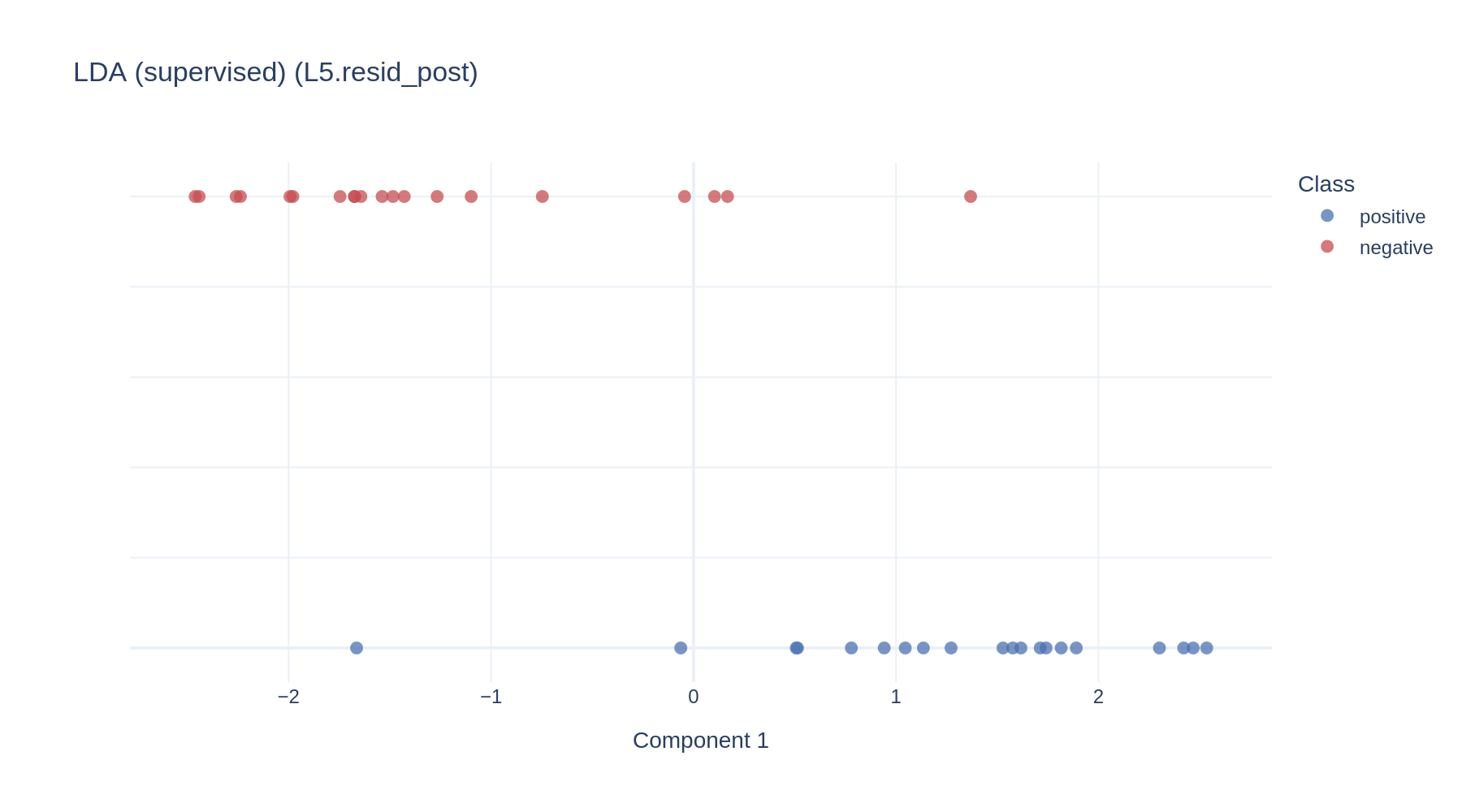

Probing: where is a concept linearly readable? figure 3

PCA is unsupervised: it never sees the labels, it just finds the two directions of greatest variance. Run it on the same activations and compare.

from sklearn.decomposition import PCA

fig = plot_activation_projection(
    store,
    probe.best_layer,
    PCA(n_components=2),
    label_names=dataset.label_names,
    title="PCA (unsupervised)",
)
save_figure(fig, f"{OUTPUT_DIR}/plots/projection_pca.png")
fig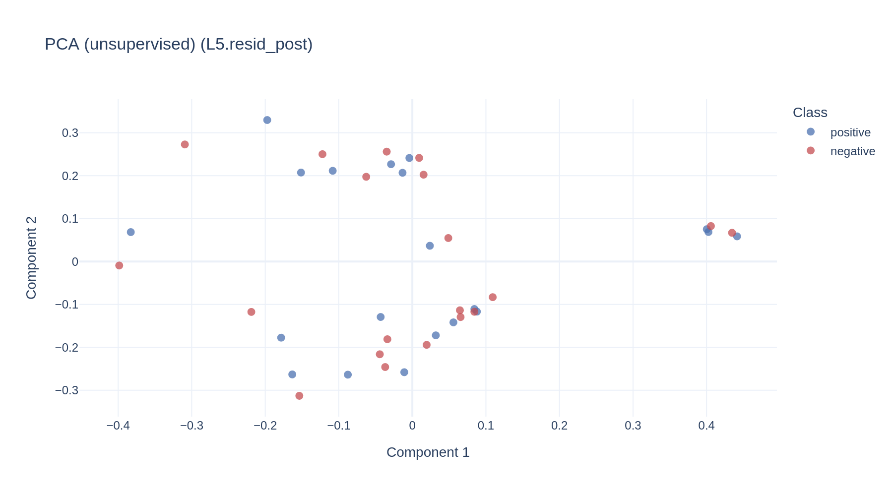

Probing: where is a concept linearly readable? figure 4

The classes are thoroughly mixed.

That is not a contradiction, and it is worth sitting with. At this layer a linear probe separates sentiment with high accuracy, so the concept is linearly decodable. But sentiment is not one of the two largest directions of variance, so PCA, which only looks for variance, walks straight past it.

Decodable and dominant are different properties. A probe measures the first. An unsupervised projection shows you the second. Reaching for PCA to “see whether the concept is there” will quietly mislead you.

5. Did the model build the concept, or was it always there?

Layer 0 is the block output immediately after the token embeddings, before any attention or MLP has run. If sentiment were assembled by the network, the probe should be near chance there.

best = probe.best_layer
print(f"layer 0  : {probe.accuracy_per_layer[0]:.3f}")
print(f"{best} : {probe.accuracy_per_layer[best]:.3f}   (best)")

layer 0  : 0.825
L5.resid_post : 0.925   (best)

It is not near chance. The probe already reads sentiment off layer 0 with high accuracy, because words like “love” and “terrible” carry the label in their token embeddings alone. The later layers do not create the concept; they sharpen a distinction that the vocabulary already supplies.

Projecting layer 0 makes the same point from the other side: the leading direction of variance is dominated by a couple of outlying sentences, and has nothing to do with the classes.

fig = plot_activation_projection(
    store,
    0,
    PCA(n_components=2),
    label_names=dataset.label_names,
    title="PCA at layer 0 (token embeddings)",
)
save_figure(fig, f"{OUTPUT_DIR}/plots/projection_pca_layer0.png")
fig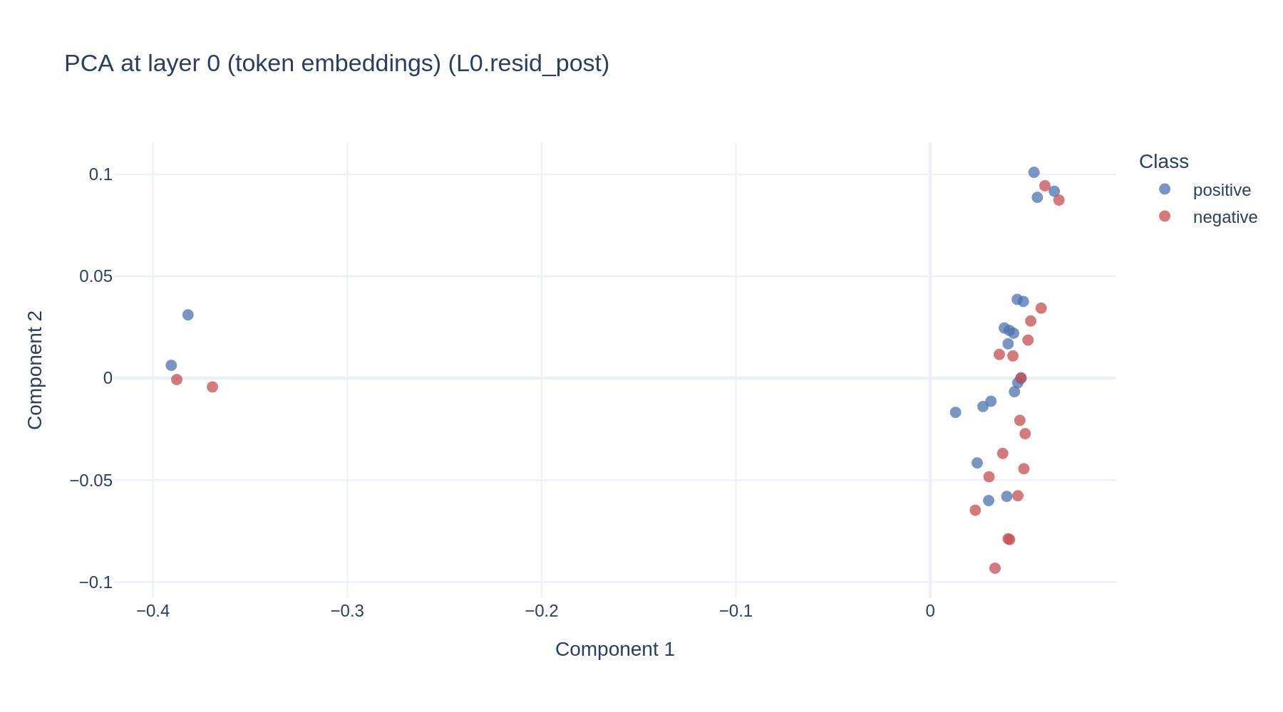

Probing: where is a concept linearly readable? figure 5

This matters beyond probing. steering.ipynb derives a direction from the same kind of data and finds that layer 0 separates the classes best of all, and yet steering there changes nothing, because eleven layers of computation overwrite it.

Readable is not the same as dominant, and neither is the same as causally effective. A probe answers only the first question.

6. Save

run_dir = Save(
    output_dir="murano_outputs", run_name="probing", model_id=model.model_id
)(results)[keys.OUTPUT_DIR]

print("saved to:", run_dir)

saved to: murano_outputs/probing

What next

steering.ipynb shows the same direction is causally usable, and that readable is not the same as effective.
custom_pipeline.ipynb plots readability against steerability, layer by layer.